from __future__ import print_function, division
import numpy as np
import matplotlib.pylab as plt
from PyAstronomy import funcFit2 as fuf2
import scipy.optimize as sco
np.random.seed(1234)
class LinMod(fuf2.MBOEv):
""" Linear model """
def __init__(self):
# 'pars' specifies parameter names in the model
fuf2.MBOEv.__init__(self, pars=["const", "slope"], rootName="LinMod")
def evaluate(self, x, *args):
"""
Evaluate model at 'x' here and return y = const + x*slope
args receives the remianing arguments specified in the call to fmin but
not needed here
"""
return self["const"] + x * self["slope"]
# Instantiate model
lm = LinMod()
lm["slope"] = 1.1
lm["const"] = -0.5
# Get some 'data' and add Gaussian noise with STD 10
x = np.arange(15.)
y = lm.evaluate(x) + np.random.normal(0,1,len(x))
yerr = np.ones_like(x)
print("Input values for mock data: ", lm.parameters())
print()
lm.thaw(["slope", "const"])
# Because ln inherited from MBOEv, it has a default chi-square objective function
fr = sco.fmin(lm.chisqr, x0=lm.freeParamVals(), args=(x,y,yerr))
lm.setFreeParamVals(fr)
lm.parameterSummary()
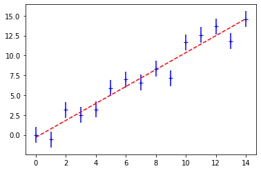
plt.errorbar(x, y, yerr=yerr, fmt='b+')
plt.plot(x, lm.evaluate(x), 'r--')
plt.show()